Hong Kong River Quality
Analysing Hong Kong Water Quality Data
By Chi Kit Yeung in R Descriptive Statistics Data Visualization
November 9, 2022
Updated: July 10, 2024
An Analysis of Hong Kong’s River Water Quality
💡 TL;DR Skip to the results
Introduction
Hong Kong prides itself in it’s ability to provide potable water directly to people’s homes straight out of the tap. But how is it down the line? In this project I want dive into the water parameter data collected from the territory’s major rivers to find out it’s current state and to learn which river is the cleanest.
Methodology
Hong Kong’s Environment Protection Department (EPD) collects 48 different physiochemical water parameters. Since these parameters cannot be directly compared with one another, the use of an index can help us effectively compare the rivers.
Water Quality Index (WQI)
Most people are familiar with AQI (air quality index) but there’s also one for water. Hong Kong’s EPD defines it’s own WQI calculation based on three parameters out of the 48: Dissolved Oxygen, Biological Oxygen Demand, and Ammonia-Nitrogen. International calculations of WQI typically uses at least 5-6 different parameters reflects upon a water’s cleanliness. Since EPD already collects such a comprehensive range of water parameters, I decided to use the international calculation that should provide a more complete look at the water’s quality.
The methods for our calculation will reference the following page 1
Parameters
- Water clarity: turbidity (NTU) and total suspended solids
- Dissolved oxygen: Dissolved oxygen concentration (mg/l);
- Oxygen demand: biochemical oxygen demand (mg/l), chemical oxygen demand (mg/l) and/or total organic carbon (mg/l);
- Nutrients: total nitrogen (mg/l), and/or total phosphorus (mg/l);
- Bacteria: total coliform (# per mg/l) and/or fecal coliform (# per mg/l).
This index’s score ranges from 0 to 100 where the lower the score, the better.1
| WQI | Rating |
|---|---|
| 0-45 | Good |
| 45-60 | Fair |
| >60 | Poor |
Feature Description
Clarity
Turbidity (NTU) - Turbidity is a fancy way of saying clarity. The cloudier the water, the more turbid it is.
Oxygen Availabilty
Dissolved Oxygen (mg/L) - DO doesn’t really represent how clean water is but the higher the DO, the better the water’s ability to purify itself by sustaining good biodiversity.
Oxygen Demand
Total Organic Carbon (mg/L), total concentration of organic carbon. Organic carbon can come from all kinds of organic matter, eg. faeces, decaying matter, etc.
5-Day Biochemical Oxygen Demand (mg/L), or BOD5 in short, measures the amount of oxygen used after a 5-day incubation period. What this represents is the amount of organic matter in the water. The lower the better.
Chemical Oxygen Demand (mg/L), or COD, is very similar to BOD5 but the incubation process is sped up using some chemical processes. This broadly represents the amount of foreign chemical substance in water.
Nutrients
Total Nitrogen (mg/L) is the sum of ammonia (found in excreted waste, i.e your pee), nitrite, nitrate, and other organic nitrogen (in proteins). Nitrite and nitrates are byproducts of ammonia that can be utilized by plants and algae.
Total Phosphorus (mg/L) - Phosphorus is an essential element for plant and algal growth. They can be found naturally in water but can also be introduced from fertilized farmland run offs. Excess phosphorus usually leads to green water (eutrophication) and explosive algae growth.
Bacteria
Faecal Coliforms (counts/100mL) - This parameter is an indicator of 💩 bacteria in the water. A high level suggests that untreated sewage/adventurous outdoor toilet goer may be leeching into the river.
Analysis
Libraries
# Metapackage of all tidyverse packages
library(tidyverse)

# Helpful data cleaning package
library(janitor)

# Date parsing
library(lubridate)

# Data visualization packages
library(ggplot2)
Importing the Dataset
df_raw <- read_csv('../input/hkriverhistorical1986-2020/river-historical-1986_2020-en.csv')
Cleaning and Wrangling
# Filtering the desired features and simplifying the names

df <- df_raw %>%
  clean_names() %>%
  filter(!is.na(river)) %>%
  subset(select = c(water_control_zone,
                    river,
                    station,
                    dates,
                    sample_no,
                    turbidity_ntu,
                    suspended_solids_mg_l,
                    dissolved_oxygen_mg_l,
                    x5_day_biochemical_oxygen_demand_mg_l,
                    chemical_oxygen_demand_mg_l,
                    total_organic_carbon_mg_l,
                    total_phosphorus_mg_l,
                    total_kjeldahl_nitrogen_mg_l,
                    faecal_coliforms_counts_100m_l
         )) %>%
rename(turbidity = turbidity_ntu,
        ss = suspended_solids_mg_l,
        dissolved_oxygen = dissolved_oxygen_mg_l,
        bod5 = x5_day_biochemical_oxygen_demand_mg_l,
        cod = chemical_oxygen_demand_mg_l,
        t_carbon = total_organic_carbon_mg_l,
        t_phosphorus = total_phosphorus_mg_l,
        t_nitrogen = total_kjeldahl_nitrogen_mg_l,
        faecal_coliform = faecal_coliforms_counts_100m_l
        ) %>%
mutate(ss = as.double(ss),
         bod5 = as.double(bod5),
         cod = as.double(cod),
         t_carbon = as.double(t_carbon),
         t_carbon = if_else(is.na(t_carbon), 0.9, t_carbon),
         t_phosphorus = as.double(t_phosphorus),
         t_phosphorus = if_else(is.na(t_phosphorus), 0.01, t_phosphorus),
         t_nitrogen = as.double(t_nitrogen),
         t_nitrogen = if_else(is.na(t_nitrogen), 0.04, t_nitrogen),
         faecal_coliform = if_else(faecal_coliform == '<1', '0.9', faecal_coliform),
         faecal_coliform = as.double(faecal_coliform))
Analysis
Getting to Know the Dataset
glimpse(df)
Rows: 31,432
Columns: 14
$ water_control_zone <chr> "Junk Bay", "Junk Bay", "Junk Bay", "Junk Bay", "Ju…
$ river              <chr> "Tseng Lan Shue Stream", "Tseng Lan Shue Stream", "…
$ station            <chr> "JR11", "JR11", "JR11", "JR11", "JR11", "JR11", "JR…
$ dates              <date> 1986-04-29, 1986-05-19, 1986-06-18, 1986-07-24, 19…
$ sample_no          <dbl> 1, 1, 1, 1, 1, 1, 1, 1, 1, 1, 1, 1, 1, 1, 1, 1, 1, …
$ turbidity          <dbl> 4.1, 4.2, 5.5, 6.5, 6.7, 3.2, 2.0, 2.3, 5.0, 24.0, …
$ ss                 <dbl> 6.5, 6.5, 8.5, 6.0, 7.0, 5.0, 3.5, 7.0, 10.0, 31.0,…
$ dissolved_oxygen   <dbl> 6.0, 5.3, 6.2, 5.2, 5.1, 5.6, 6.9, 6.7, 7.7, 0.8, 3…
$ bod5               <dbl> 9.7, 5.6, 9.0, 12.2, 8.8, 2.1, 5.9, 8.0, 9.0, 113.3…
$ cod                <dbl> 13, 21, 19, 17, 5, 5, 29, 160, 46, 66, 83, 45, 12, …
$ t_carbon           <dbl> 0.9, 5.0, 1.0, 0.9, 5.0, 4.0, 0.9, 0.9, 7.0, 10.0, …
$ t_phosphorus       <dbl> 2.50, 2.00, 1.90, 2.10, 4.50, 1.20, 3.80, 6.80, 5.7…
$ t_nitrogen         <dbl> 4.1, 5.1, 3.1, 5.5, 5.3, 1.1, 2.7, 12.0, 20.0, 18.0…
$ faecal_coliform    <dbl> NA, NA, NA, NA, NA, NA, NA, NA, NA, NA, NA, NA, NA,…
# List of Rivers in the Dataset
sort(unique(df$river))
'Fairview Park Nullah''Ha Pak Nai Stream''Ho Chung River''Kai Tak River''Kam Tin River''Kau Wa Keng Stream''Kwun Yam Shan Stream''Lam Tsuen River''Mui Wo River''Ngau Hom Sha Stream''Pai Min Kok Stream''Pak Nai Stream''River Beas''River Ganges''River Indus''Sam Dip Tam Stream''Sha Kok Mei Stream''Shan Liu Stream''Sheung Pak Nai Stream''Shing Mun River''Siu Lek Yuen Nullah''Tai Chung Hau Stream''Tai Po Kau Stream''Tai Po River''Tai Shui Hang Stream''Tai Wai Nullah''Tin Shui Wai Nullah''Tin Sum Nullah''Tsang Kok Stream''Tseng Lan Shue Stream''Tuen Mun River''Tung Chung River''Tung Tze Stream''Yuen Long Creek'
# Number of Rivers in Dataset
length(unique(df$river))
34
Calculate WQI Subindexes
# Calculate subindex (si)
index_df <- df %>%
  mutate(turbidity_si = case_when(
    turbidity <= 1.5 ~ 10,
    turbidity > 1.5 & turbidity <= 3.0 ~ 20,
    turbidity > 3.0 & turbidity <= 4.0 ~ 30,
    turbidity > 4.0 & turbidity <= 4.5 ~ 40,
    turbidity > 4.5 & turbidity <= 5.2 ~ 50,
    turbidity > 5.2 & turbidity <= 8.8 ~ 60,
    turbidity > 8.8 & turbidity <= 12.2 ~ 70,
    turbidity > 12.2 & turbidity <= 16.5 ~ 80,
    turbidity > 16.5 & turbidity <= 21 ~ 90,
    turbidity > 21 ~ 100
  )) %>%
  mutate(ss_si = case_when(
    ss <= 2 ~ 10,
    ss > 2 & ss <= 3 ~ 20,
    ss > 3 & ss <= 4 ~ 30,
    ss > 4 & ss <= 5.5 ~ 40,
    ss > 5.5 & ss <= 6.5 ~ 50,
    ss > 6.5 & ss <= 9.5 ~ 60,
    ss > 9.5 & ss <= 12.5 ~ 70,
    ss > 12.5 & ss <= 18 ~ 80,
    ss > 18 & ss <= 26.5 ~ 90,
    ss > 26.5 ~ 100
  )) %>%
  mutate(dissolved_oxygen_si = case_when(
    dissolved_oxygen >= 8 ~ 10,
    dissolved_oxygen < 8 & dissolved_oxygen >= 7.3 ~ 20,
    dissolved_oxygen < 7.3 & dissolved_oxygen >= 6.7 ~ 30,
    dissolved_oxygen < 6.7 & dissolved_oxygen >= 6.3 ~ 40,
    dissolved_oxygen < 6.3 & dissolved_oxygen >= 5.8 ~ 50,
    dissolved_oxygen < 5.8 & dissolved_oxygen >= 5.3 ~ 60,
    dissolved_oxygen < 5.3 & dissolved_oxygen >= 4.8 ~ 70,
    dissolved_oxygen < 4.8 & dissolved_oxygen >= 4 ~ 80,
    dissolved_oxygen < 4 & dissolved_oxygen >= 3.1 ~ 90,
    dissolved_oxygen < 3.1 ~ 100
  )) %>%
  mutate(bod5_si = case_when(
    bod5 <= 0.8 ~ 10,
    bod5 > 0.8 & bod5 <= 1 ~ 20,
    bod5 > 1 & bod5 <= 1.1 ~ 30,
    bod5 > 1.1 & bod5 <= 1.3 ~ 40,
    bod5 > 1.3 & bod5 <= 1.5 ~ 50,
    bod5 > 1.5 & bod5 <= 1.9 ~ 60,
    bod5 > 1.9 & bod5 <= 2.3 ~ 70,
    bod5 > 2.3 & bod5 <= 3.3 ~ 80,
    bod5 > 3.3 & bod5 <= 5.1 ~ 90,
    bod5 > 5.1 ~ 100
  )) %>%
  mutate(cod_si = case_when(
    cod <= 16 ~ 10,
    cod > 16 & cod <= 24 ~ 20,
    cod > 24 & cod <= 32 ~ 30,
    cod > 32 & cod <= 38 ~ 40,
    cod > 38 & cod <= 46 ~ 50,
    cod > 46 & cod <= 58 ~ 60,
    cod > 58 & cod <= 72 ~ 70,
    cod > 72 & cod <= 102 ~ 80,
    cod > 102 & cod <= 146 ~ 90,
    cod > 146 ~ 100
  )) %>%
  mutate(t_carbon_si = case_when(
    t_carbon <= 5 ~ 10,
    t_carbon > 5 & t_carbon <= 7 ~ 20,
    t_carbon > 7 & t_carbon <= 9.5 ~ 30,
    t_carbon > 9.5 & t_carbon <= 12 ~ 40,
    t_carbon > 12 & t_carbon <= 14 ~ 50,
    t_carbon > 14 & t_carbon <= 17.5 ~ 60,
    t_carbon > 17.5 & t_carbon <= 21 ~ 70,
    t_carbon > 21 & t_carbon <= 27.5 ~ 80,
    t_carbon > 27.5 & t_carbon <= 37 ~ 90,
    t_carbon > 37 ~ 100
  )) %>%
  mutate(t_nitrogen_si = case_when(
    t_nitrogen <= 0.55 ~ 10,
    t_nitrogen > 0.55 & t_nitrogen <= 0.75 ~ 20,
    t_nitrogen > 0.75 & t_nitrogen <= 0.9 ~ 30,
    t_nitrogen > 0.9 & t_nitrogen <= 1 ~ 40,
    t_nitrogen > 1 & t_nitrogen <= 1.2 ~ 50,
    t_nitrogen > 1.2 & t_nitrogen <= 1.4 ~ 60,
    t_nitrogen > 1.4 & t_nitrogen <= 1.6 ~ 70,
    t_nitrogen > 1.6 & t_nitrogen <= 2 ~ 80,
    t_nitrogen > 2 & t_nitrogen <= 2.7 ~ 90,
    t_nitrogen > 2.7 ~ 100
  )) %>%
  mutate(t_phosphorus_si = case_when(
    t_phosphorus <= 0.02 ~ 10,
    t_phosphorus > 0.02 & t_phosphorus <= 0.03 ~ 20,
    t_phosphorus > 0.03 & t_phosphorus <= 0.05 ~ 30,
    t_phosphorus > 0.05 & t_phosphorus <= 0.07 ~ 40,
    t_phosphorus > 0.07 & t_phosphorus <= 0.09 ~ 50,
    t_phosphorus > 0.09 & t_phosphorus <= 0.16 ~ 60,
    t_phosphorus > 0.16 & t_phosphorus <= 0.24 ~ 70,
    t_phosphorus > 0.24 & t_phosphorus <= 0.46 ~ 80,
    t_phosphorus > 0.46 & t_phosphorus <= 0.89 ~ 90,
    t_phosphorus > 0.89 ~ 100
  )) %>%
  mutate(faecal_coliform_si = case_when(
    faecal_coliform <= 10 ~ 10,
    faecal_coliform > 10 & faecal_coliform <= 20 ~ 20,
    faecal_coliform > 20 & faecal_coliform <= 35 ~ 30,
    faecal_coliform > 35 & faecal_coliform <= 55 ~ 40,
    faecal_coliform > 55 & faecal_coliform <= 75 ~ 50,
    faecal_coliform > 75 & faecal_coliform <= 135 ~ 60,
    faecal_coliform > 135 & faecal_coliform <= 190 ~ 70,
    faecal_coliform > 190 & faecal_coliform <= 470 ~ 80,
    faecal_coliform > 470 & faecal_coliform <= 960 ~ 90,
    faecal_coliform > 960 ~ 100,
    is.na(faecal_coliform) ~ 50
  ))

head(index_df)
# Calculate WQI
index_df$wqi <- round(
    rowMeans(subset(index_df,
                    select = c(
                        turbidity_si,
                        ss_si,
                        dissolved_oxygen_si,
                        bod5_si,
                        cod_si,
                        t_carbon_si,
                        t_nitrogen_si,
                        t_phosphorus_si,
                        faecal_coliform_si)),
             na.rm = TRUE))

river <- index_df %>%
  mutate(year = year(dates)) %>%
  mutate(month = month(dates)) %>%
  subset(select = c(water_control_zone, river, station, year, month, wqi)) %>%
  group_by(water_control_zone, river, year) %>%
  summarise(wqi = round(mean(wqi)))

head(river)
Results
Overview
# Plot size
options(repr.plot.width=15, repr.plot.height=10)
# Convert data from long format to wide
wide <- river %>%
spread(year, wqi)
wide$average <- round(rowMeans(subset(wide, select = -c(water_control_zone, river)), na.rm = TRUE))
# Sort entries by Average WQI
wide <- wide %>%
arrange(average)
categorized <- wide %>%
mutate(quality = case_when(
average >= 0 & average < 45 ~ 'good',
average >= 45 & average < 60 ~ 'fair',
average >= 60 ~ 'poor'
))
p <- categorized %>%
group_by(quality) %>%
tally() %>%
ggplot(mapping = aes(x = reorder(quality, -n), y = n, fill = quality)) +
scale_fill_manual(values = c("aquamarine4", "cyan", "chocolate4")) +
geom_col(width = 1) +
geom_text(aes(y = n+1, label = paste(n, " | (", round(n/sum(n)*100, 2),"%", ")", sep = ""), size = 50)) +
geom_text(aes(y = n-1, label = c("Fair", "Good", "Poor")), size = 15) +
geom_text(aes(y = n-1.5, label = paste(round(n/sum(n)*100, 2),"%"), size = 1)) +
theme_bw()
p +
theme(
panel.grid = element_blank(),
title = element_text(size = 20, face = "bold"),
plot.subtitle = element_text(size = 15, face = "bold"),
# axis.text.x = element_text(size = 14, face = "bold"),
plot.caption = element_text(size = 10),
axis.text = element_blank(),
axis.ticks = element_blank(),
panel.border = element_blank(),
legend.position = "none"
) +
labs(
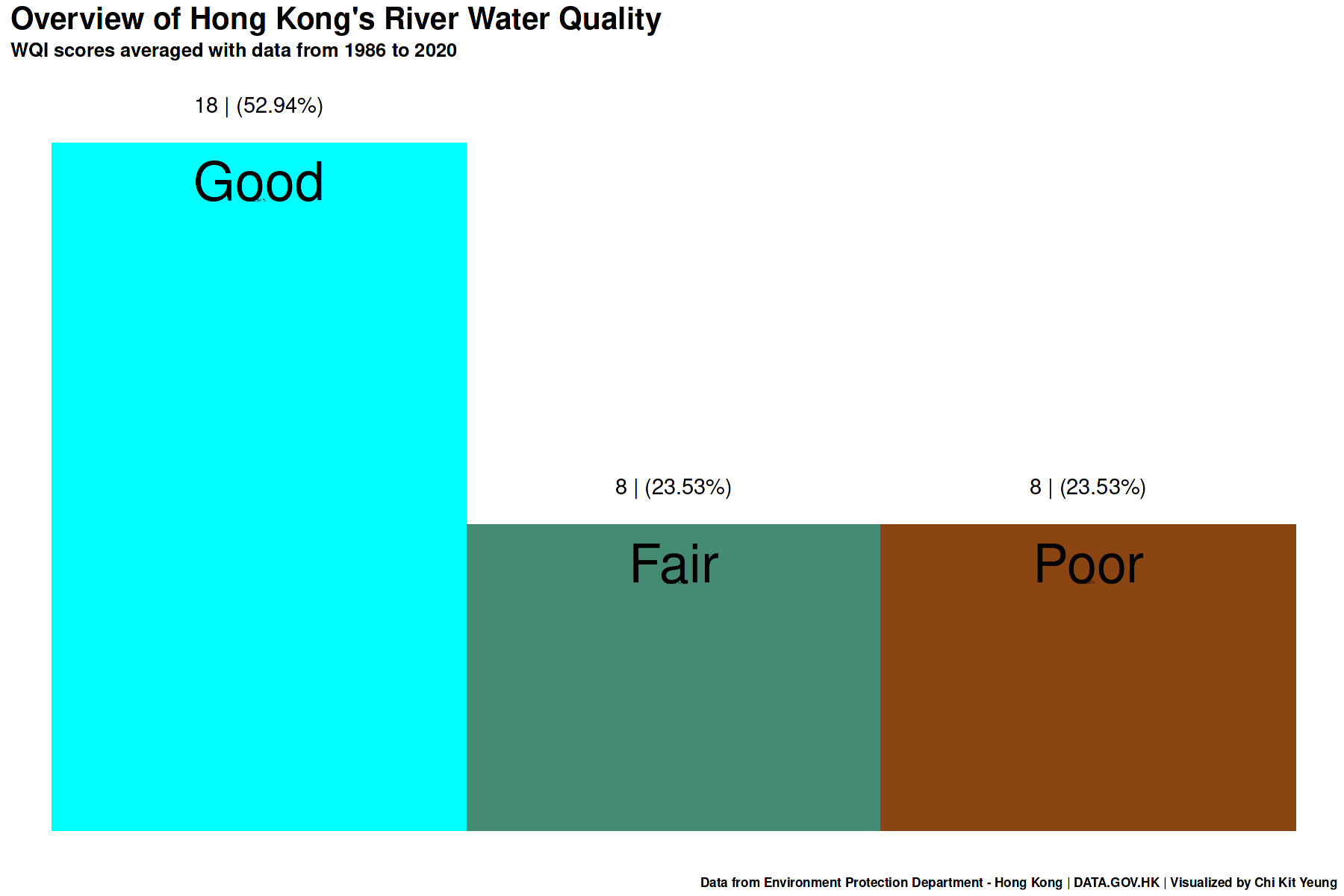
title = "Overview of Hong Kong's River Water Quality",
subtitle = "WQI scores averaged with data from 1986 to 2020",
caption = "Data from Environment Protection Department - Hong Kong | DATA.GOV.HK | Visualized by Chi Kit Yeung",
x = NULL,
y = NULL
)
# p
What this means?
- On average, over half of all the rivers being monitored (18) are considered to have good water quality (52.94%)
- The remaining are split equally between rivers with fair water quality (8) and poor water quality (8).
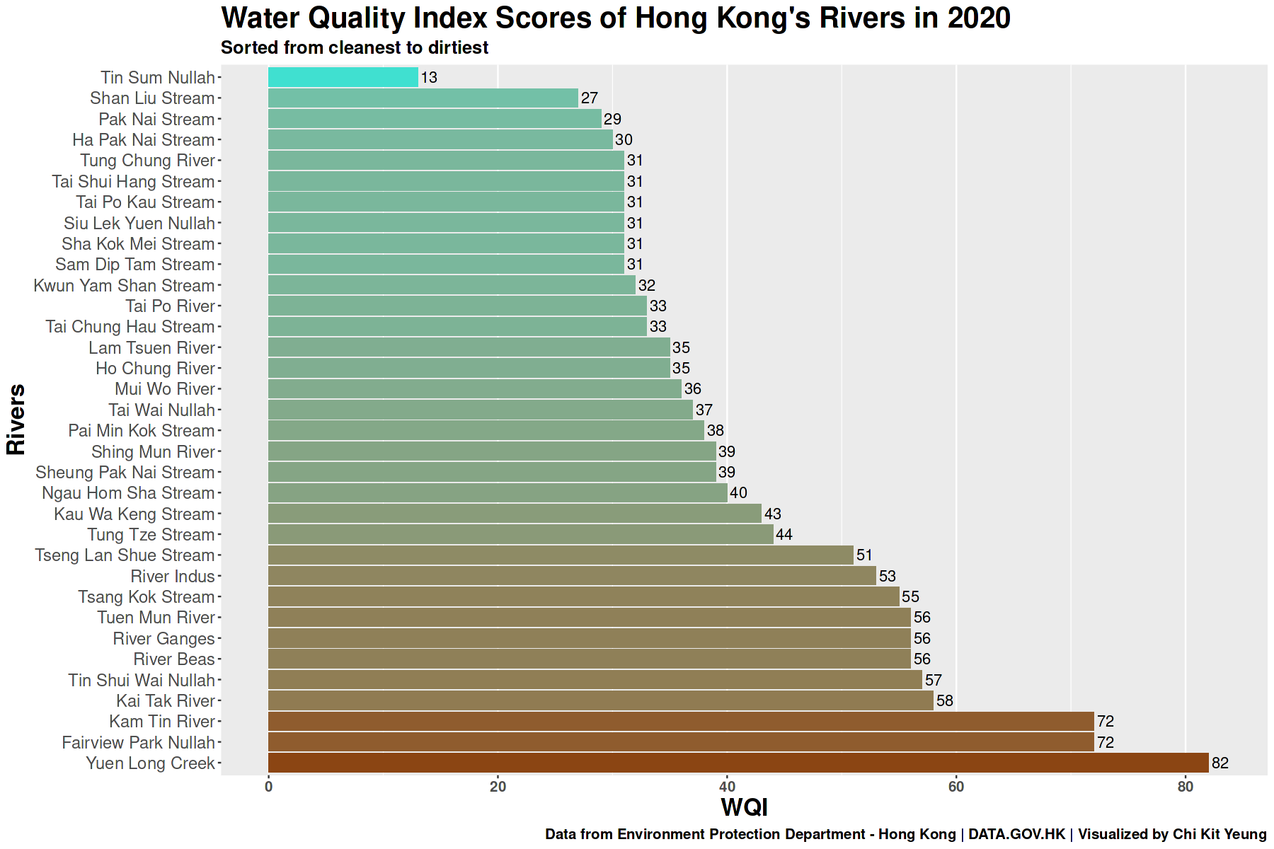
Which river is cleanest? Which is worst?
First let’s take a look at the latest available data from 2020. We can compare the WQI scores from each river and see which is the highest, the lowest, and every one in between.
# Bar Plot
b <- river %>%
  filter(year == 2020) %>%
  ggplot(mapping = aes(y = reorder(river, -wqi), x = wqi, fill = wqi)) +
  geom_col() +
  geom_text(aes(label = wqi, x = wqi+1, size = 14))

b +
  scale_fill_gradient(low="turquoise", high="chocolate4", na.value = NA) +
#   theme_bw() +
  theme(
    title = element_text(size = 20, face = "bold"),
    plot.subtitle = element_text(size = 15, face = "bold"),
    plot.caption = element_text(size = 12),
    axis.text.y = element_text(size = 14),
    axis.text.x = element_text(size = 12, face = "bold"),
    panel.grid.major.y = element_blank(),
    legend.position = "none"
  ) +
  labs(
    title = "Water Quality Index Scores of Hong Kong's Rivers in 2020",
    subtitle = "Sorted from cleanest to dirtiest",
    caption = "Data from Environment Protection Department - Hong Kong | DATA.GOV.HK | Visualized by Chi Kit Yeung",
    x = "WQI",
    y = "Rivers"
  )
What this means?
- Based on latest available data, Tin Sum Nullah is the cleanest river in Hong Kong
- Yuen Long Creek is the dirtiest river
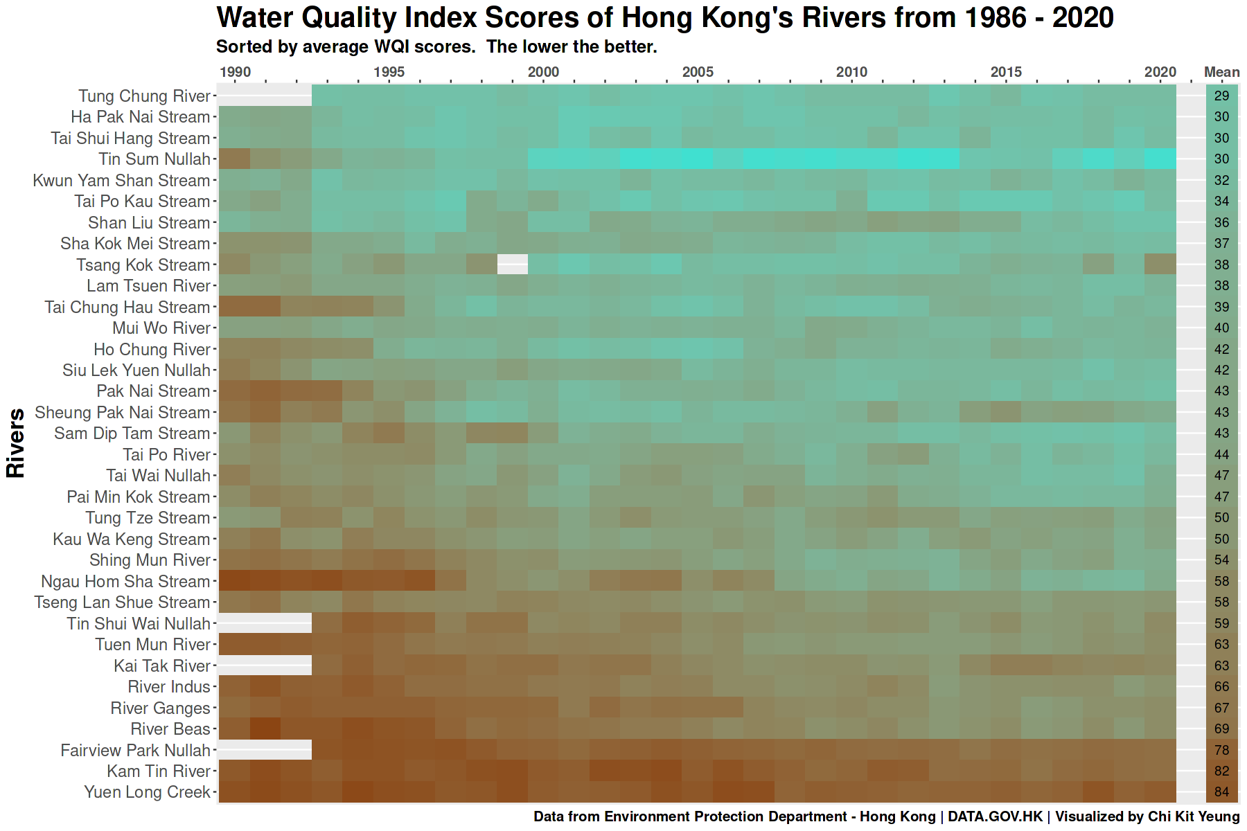
Which river is consistently cleaner?
# Heat Map

# Convert data back to long format for visualization
long <- wide %>%
  # Just a place holder to create gap in viz
  add_column('2021' = NA) %>%
  pivot_longer(cols = !c(water_control_zone, river), names_to = 'year', values_to = 'wqi')

# Vectors to serve as custom ordering and label for the viz
order <- c(rev(unique(long$river)))
x_label <- c()
for (i in 1990:2020) {
  if (i %% 5 == 0) {
    x_label <- append(x_label, i)
  } else {
    x_label <- append(x_label, "")
  }
}

# Begin Viz
h <- ggplot(mapping = aes(x = year, y = river)) +
  geom_tile(aes(fill = wqi), long) +
  geom_text(aes(label = wqi), subset(long, year == "average")) +
  scale_x_discrete(limits = c(1990:2021, "average"), labels = c(x_label, "", "Mean"), position = "top") +
  scale_y_discrete(limits = order)

# Finishing touches
h +
  scale_fill_gradient(low="turquoise", high="chocolate4", na.value = NA) +
  guides(colour = guide_colorbar(reverse = TRUE)) +
#   theme_bw() +
  theme(
    panel.grid.major.x = element_blank(),
    title = element_text(size = 20, face = "bold"),
    plot.subtitle = element_text(size = 15, face = "bold"),
    plot.caption = element_text(size = 12),
    axis.text.y = element_text(size = 14),
    axis.text.x = element_text(size = 12, face = "bold"),
    legend.position = "none"
  ) +
  labs(
    title = "Water Quality Index Scores of Hong Kong's Rivers from 1986 - 2020",
    subtitle = "Sorted by average WQI scores.  The lower the better.",
    caption = "Data from Environment Protection Department - Hong Kong | DATA.GOV.HK | Visualized by Chi Kit Yeung",
    x = NULL,
    y = "Rivers"
  )
What this means?
- Most river’s water quality has improved over the past decades
- Tung Chung River has consistently been the cleanest with an average WQI of 29
- Yuen Long Creek maintains it position as the worst river in Hong Kong, it consistenly had poor water quality over the past decades
Conclusions
- On average, over half of all the rivers being monitored (18) are considered to have good water quality (52.94%)
- The remaining are split equally between rivers with fair water quality (8) and poor water quality (8).
- Based on latest available data, Tin Sum Nullah is the cleanest river in Hong Kong (WQI of 13)
- Yuen Long Creek is the dirtiest river (WQI 82)
- Most river’s water quality has improved over the past decades
- Tung Chung River has consistently been the cleanest with an average WQI of 29
- Yuen Long Creek maintains it position as the worst river in Hong Kong, it consistenly had poor water quality over the past decades
Hypothesis for future analysis
Like most things in the world, I think that the cause of dirty rivers can probably be linked back to anthropogenic interference. In order to verify this I will need data on each river’s proximity to urban areas or some way to quantify their exposure to urban factors.
Future Analysis
- Determine which river has improved the most
- Which river is the poopiest 💩 (fecal coliform & e.coli parameters)
- Comparison of water quality in the 90s to now
🎉 Thank you for reading! Please feel to give suggestions, share your thoughts, or just say Hi
- Posted on:
- November 9, 2022
- Length:
- 14 minute read, 2827 words
- Categories:
- R Descriptive Statistics Data Visualization
- See Also: