Inferential Statistics
How to Perform Inferential Statistics in R
By Chi Kit Yeung in Statistics R
January 13, 2023
Distributions
Normal Distribution
Standard Normal Distribution
Standardization can be applied to any distribution. A standardized normal distribution will have a mean of 0 and a standard deviation of 1.
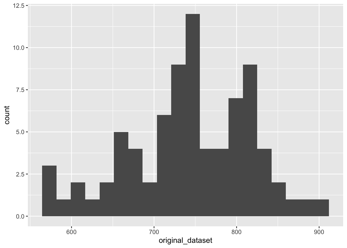
Data Set
original_dataset <- c(567.45, 572.45, 572.45, 589.12, 613.87, 615.78, 628.45, 644.87, 650.45, 652.20, 656.87, 661.45, 666.45, 667.70, 668.95, 675.28, 675.78, 685.53, 694.28, 697.62, 705.78, 705.87, 708.12, 711.03, 714.03, 716.03, 722.28, 728.12, 728.70, 729.03, 730.12, 731.95, 735.03, 736.95, 737.37, 738.28, 739.78, 740.62, 743.62, 747.20, 748.20, 748.28, 748.53, 750.03, 752.12, 754.70, 755.03, 758.37, 760.53, 764.03, 769.28, 775.45, 781.20, 781.70, 785.62, 792.78, 793.37, 795.28, 797.62, 798.95, 799.70, 799.95, 810.87, 811.53, 813.62, 814.03, 814.78, 817.87, 818.87, 820.70, 821.12, 825.62, 828.62, 841.45, 842.03, 842.87, 849.62, 874.70, 878.78, 897.45)

ggplot(mapping = aes(original_dataset)) +
  geom_histogram(bins = 20)
Calculate the mean and standard deviation of the dataset
mean <- mean(original_dataset)
standard_deviation <- sd(original_dataset)

mean
## [1] 743.027
standard_deviation
## [1] 73.95317
Standardize the dataset
The formula
$$z=\frac{x-\mu}{\sigma}$$
standardized_dataset <- (original_dataset-mean)/standard_deviation

standardized_dataset
##  [1] -2.374164556 -2.306554204 -2.306554204 -2.081141291 -1.746470048
##  [6] -1.720642893 -1.549318261 -1.327285865 -1.251832712 -1.228169089
## [11] -1.165021020 -1.103089938 -1.035479586 -1.018576998 -1.001674410
## [16] -0.916079704 -0.909318669 -0.777478482 -0.659160366 -0.613996651
## [21] -0.503656557 -0.502439570 -0.472014912 -0.432665687 -0.392099476
## [26] -0.365055335 -0.280542395 -0.201573504 -0.193730703 -0.189268420
## [31] -0.174529363 -0.149783974 -0.108135997 -0.082173622 -0.076494352
## [36] -0.064189268 -0.043906163 -0.032547623  0.008018588  0.056427600
## [41]  0.069949670  0.071031436  0.074411953  0.094695059  0.122956186
## [46]  0.157843128  0.162305411  0.207469126  0.236676798  0.284004045
## [51]  0.354994914  0.438426089  0.516177994  0.522939029  0.575945545
## [56]  0.672763569  0.680741591  0.706568745  0.738210390  0.756194744
## [61]  0.766336296  0.769716814  0.917377823  0.926302389  0.954563516
## [66]  0.960107565  0.970249118  1.012032316  1.025554386  1.050299775
## [71]  1.055979045  1.116828361  1.157394573  1.330882736  1.338725537
## [76]  1.350084076  1.441358051  1.780491577  1.835661624  2.088118679
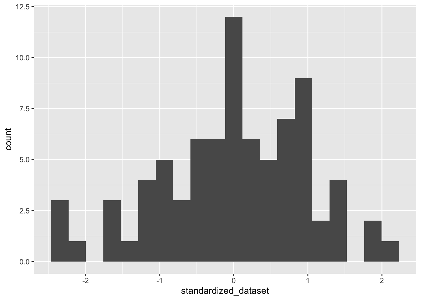
Now that we have the new standardized dataset let’s try plotting it
new_mean <- mean(standardized_dataset)
new_standard_deviation <- sd(standardized_dataset)

round(new_mean)
## [1] 0
round(new_standard_deviation)
## [1] 1
Plot the data on a graph to see the change
ggplot(mapping = aes(standardized_dataset)) +
  geom_histogram(bins = 20)
Central Limit Theorem
Standard Error
Confidence Interval
Single Population
z-Statistic
$$CI = \overline{x} \pm z_{\alpha/2} \frac{\sigma}{\sqrt{n}}$$
Dataset
Given:
dataScientist_salaries <- c(117313, 104002, 113038, 101936, 84560, 113136, 80740, 100536, 105052, 87201, 91986, 94868, 90745, 102848, 85927, 112276, 108637, 96818, 92307, 114564, 109714, 108833, 115295, 89279, 81720, 89344, 114426, 90410, 95118, 113382)

std_dev <- 15000
Population Standard deviation = $15,000
Calculate the mean
salary_mean <- mean(dataScientist_salaries)
salary_mean
## [1] 100200.4
Find the appropriate z-score for calculating a 90% confidence interval
R has a couple of handy functions to find the z distribution values. First is the pnorm() which receives the z-value and spits back out the \(\alpha\)/2 value.
# 95% Confidence Interval, z0.025
pnorm(1.96)
## [1] 0.9750021
# 99% Confidence Interval, z 0.005
qnorm(0.995)
## [1] 2.575829
Knowing this, to get the z-value for a 90% confidence interval estimate. The alpha is 1-0.9, or 0.1. Divide that by 2 to get \(\alpha\)/2 and we’ll need to get the z-value for 1-0.05, 0.95.
z <- qnorm(0.95)
z
## [1] 1.644854
I find this whole thing unnecessarily complex. Let’s make a small function to get the results by simply inputting the desired confidence interval
confidence <- 90

z <- round(qnorm(1-(1-(confidence/100))/2), 2)
lower_int <- round(salary_mean - z*(std_dev/sqrt(30)))

upper_int <- round(salary_mean + z*(std_dev/sqrt(30)))
Now we can say with 90% confidence that the average salary for data scientists fall between 95709 and 104692.
Student’s T Distribution
Developed by a research for Guiness beer
Dataset
t_dataset <- c(78000, 90000, 75000, 117000, 105000, 96000, 89500, 102300, 80000)
Calculate the mean and the standard error of the dataset
t_mean <- mean(t_dataset)
t_sd <- sd(t_dataset)
Determine which statistic to use for inference
If population standard deviation is not known, we should use the t-statistic. If it is known, then we will use the z-statistic.
Find the appropriate statistic, taking into consideration the degrees of freedom (if applicable) for 99% confidence
The degrees of freedom is equal to the sample size minus one
# Find df with R
t_df <- length(t_dataset)-1
t_df
## [1] 8
Like the z-value, R also has a handy function that can help find the t-statistic. pt() and qt()
# Getting the t-statistic
# 99% confidence interval
t_value <- round(qt(1-0.01/2, t_df), 2)
t_value
## [1] 3.36
Find the 99% confidence interval
Formula:
$$CI = \overline{x} \pm t_{n-1, \alpha/2} \frac{s}{\sqrt{n}}$$
lower_int <- round(t_mean - t_value*(t_sd/sqrt(length(t_dataset))))

upper_int <- round(t_mean + t_value*(t_sd/sqrt(length(t_dataset))))
Using the t-statistic, we can say with 99% confidence that the average salary for data scientists fall between 76930 and 108137.
Two Variables
Dependent Variables
Background
The 365 team has developed a diet and an exercise program for losing weight. It seems that it works like a charm. However, you are interested in how much weight are you likely to lose.
We’re provided with the following dataset:
subject <- c(1:10)
weight_before <- c(228.58, 244.01, 262.46, 224.32, 202.14, 246.98, 195.86, 231.88, 243.32, 266.74)
weight_after <- c(204.74, 223.95, 232.94, 212.04, 191.74, 233.47, 177.60, 213.85, 218.85, 236.86)

weight_loss_df <- data.frame(subject, weight_before, weight_after)
kable(weight_loss_df)
| subject | weight_before | weight_after |
|---|---|---|
| 1 | 228.58 | 204.74 |
| 2 | 244.01 | 223.95 |
| 3 | 262.46 | 232.94 |
| 4 | 224.32 | 212.04 |
| 5 | 202.14 | 191.74 |
| 6 | 246.98 | 233.47 |
| 7 | 195.86 | 177.60 |
| 8 | 231.88 | 213.85 |
| 9 | 243.32 | 218.85 |
| 10 | 266.74 | 236.86 |
Adding a new column to find the difference:
df <- weight_loss_df %>%
  mutate("difference" = weight_after-weight_before)

kable(df)
| subject | weight_before | weight_after | difference |
|---|---|---|---|
| 1 | 228.58 | 204.74 | -23.84 |
| 2 | 244.01 | 223.95 | -20.06 |
| 3 | 262.46 | 232.94 | -29.52 |
| 4 | 224.32 | 212.04 | -12.28 |
| 5 | 202.14 | 191.74 | -10.40 |
| 6 | 246.98 | 233.47 | -13.51 |
| 7 | 195.86 | 177.60 | -18.26 |
| 8 | 231.88 | 213.85 | -18.03 |
| 9 | 243.32 | 218.85 | -24.47 |
| 10 | 266.74 | 236.86 | -29.88 |
| Now that we’ve calculated the ‘difference’, we can treat this as a single population. |
We’ll be using the t-statistics because of the small (<30) sample size and unknown population variance.
# Calculating the mean and standard deviation
mean <- mean(df$difference)
sd <- sd(df$difference)

# Finding the t-statistic for a 95% confidence interval
t_value <- qt(1-0.05/2, length(df)-1)

# Calculating the confidence interval
lower_limit <- mean-t_value*(sd/sqrt(10))
upper_limit <- mean+t_value*(sd/sqrt(10))
Results:
- Mean = -20.025
- Standard deviation = 6.8617754
\(t_{9,\ 0.025}\)= t_value
\(T_{95\%}\) Confidence interval: -26.930539 and -13.119461
Inferences
- In 95% of subjects, the true mean will fall within the above interval.
- The whole interval is negative.
- All subjects successfully lost weight.
“I am 95% confident that by following the diet and exercise program you will lose between 13 to 27 lbs.”
Extra
Let’s try calculating the 90% and 99% confidence interval to see the differences.
# Creating a helper function to avoid redundant typing
find_lower_CI <- function(c) {
  round(mean-(qt(1-(1-(c/100))/2, length(df)-1))*(sd/sqrt(10)), 2)
}

find_upper_CI <- function(c) {
  round(mean+(qt(1-(1-(c/100))/2, length(df)-1))*(sd/sqrt(10)), 2)
}

# Putting the CIs in a dataframe
CI <- c("Lower Int", "Upper Int")
T90 <- c(find_lower_CI(90), find_upper_CI(90))
T95 <- c(find_lower_CI(95), find_upper_CI(95))
T99 <- c(find_lower_CI(99), find_upper_CI(99))

kable(data.frame(CI, T90, T95, T99))
| CI | T90 | T95 | T99 |
|---|---|---|---|
| Lower Int | -25.13 | -26.93 | -32.70 |
| Upper Int | -14.92 | -13.12 | -7.35 |
We can clearly see that the higher the confidence the wider the interval range. There is a trade off between higher confidence. On one hand the inference we make will very likely be correct but the range would be so wide that it is useless for any meaninful statistic.
Independent Variables
Variance of differences
z-statistic
$$ \sigma^2_x, \sigma^2_y = \frac{\sigma^2_x}{n_x} + \frac{\sigma^2_y}{n_y} $$
t-statistic
$$ s^2_p = \frac{(n_x-1)s^2_x+(n_y-1)s^2_y}{n_x+n_y-2} $$
CI Formulas
z-statistic
$$ CI = (\overline{x}-\overline{y}) \pm z_{\alpha/2} \sqrt{\frac{\sigma^2_x}{n_x} + \frac{\sigma^2_y}{n_y}}$$
t-statistic
$$ CI = (\overline{x}-\overline{y}) \pm t_{n_x+n_y-2,\alpha/2} \sqrt{\frac{s^2_p}{n_x} + \frac{s^2_p}{n_y}}$$
Excercise 1
Confidence interval for difference of two means; independent samples, variances unknown but assumed to be equal
# Dataset
ny_apple <- c(3.80, 3.76, 3.87, 3.99, 4.02, 4.25, 4.13, 3.98, 3.99, 3.62)
la_apple <- c(3.02, 3.22, 3.24, 3.02, 3.06, 3.15, 3.81, 3.44)
Since the population variance is unknown and the sample size is small, we will be using the t-statistic again for this particular excercise.
Calculation
# Find mean, standard deviation, variance
ny_mean <- mean(ny_apple)
ny_sd <- sd(ny_apple)
ny_var <- var(ny_apple)
la_mean <- mean(la_apple)
la_sd <- sd(la_apple)
la_var <- var(la_apple)
ny_len <- length(ny_apple)
la_len <- length(la_apple)

# Pooled Variance
s2p <- ((ny_var*(ny_len-1))+(la_var*(la_len-1)))/(ny_len+la_len-2)


# Find t-values
t_90 <- round(qt(1-(1-(90/100))/2, ny_len+la_len-2), 2)
t_95 <- round(qt(1-(1-(95/100))/2, ny_len+la_len-2), 2)

# Calculate CI
lower_int <- round((ny_mean-la_mean)-t_90*sqrt((s2p/ny_len)+(s2p/la_len)), 2)
upper_int <- round((ny_mean-la_mean)+t_90*sqrt((s2p/ny_len)+(s2p/la_len)), 2)
CI = (0.51, 0.88)
Excercise 2
Confidence interval for the difference of two means. Independent samples, variance known
# Dataset
index <- c("Sample Size", "Sample Mean", "Population Std")
engineering <- c(100, 58, 10)
management <- c(70, 65, 5)
difference <- c(NA, -7, 1.16)

data <- data.frame(index, engineering, management, difference)
data
##            index engineering management difference
## 1    Sample Size         100         70         NA
## 2    Sample Mean          58         65      -7.00
## 3 Population Std          10          5       1.16
We’ve pretty much been handed all the information needed on a silver platter here. Since we know the population standard deviation, we will be using the z-statistic.
Calculation
# Find z-value
z_value <- round(qnorm(1-(1-(99/100))/2), 2)

# Calculate CI
lower_int <- round(data$difference[2]-z_value*sqrt((data$engineering[3]^2/data$engineering[1])+(data$management[3]^2/data$management[1])), 2)
upper_int <- round(data$difference[2]+z_value*sqrt((data$engineering[3]^2/data$engineering[1])+(data$management[3]^2/data$management[1])), 2)
CI = (-10.01, -3.99)